Gap-aware time, frequency, and state analysis

Use this workflow when the scientific question concerns oscillatory or repeating structure in one processed photometry signal: autocorrelation, power spectral density (PSD), a time-resolved spectrogram, or differences between externally defined states.

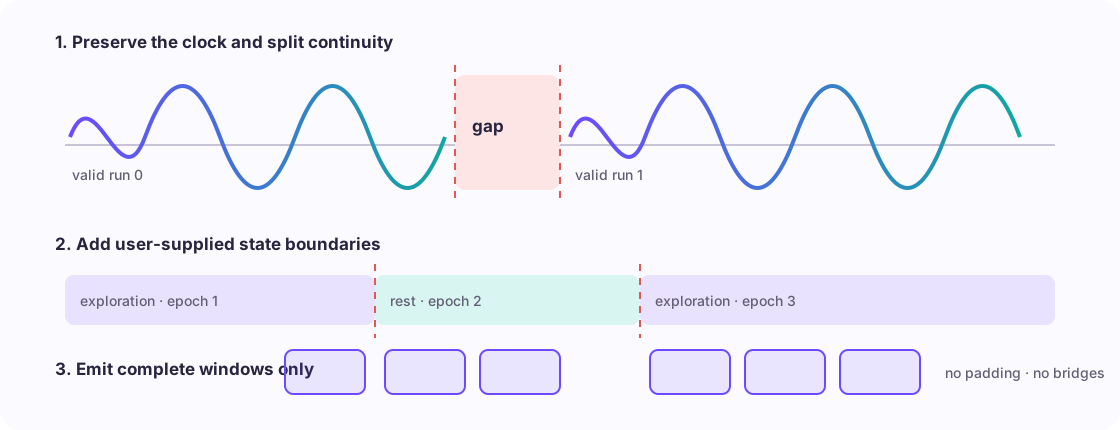
This is an experimental product API. Its central promise is operational: missing samples, timestamp gaps, and state boundaries do not become invisible signal continuity.

Every estimate is assembled from bounded evidence. Autocorrelation pairs and spectral windows stay within a regular valid run. State-conditioned workflows add user-declared epoch boundaries; they never join equal labels across separate epochs.

What is available

Question	Function	Primary evidence
Does the signal repeat at a lag?	autocorrelation	pairs per lag and continuity runs
Where is power concentrated?	welch_psd	windows per run and power-density units
How does frequency content change?	spectrogram	every window's bounds, run, and edge distances
Does any of the above differ by supplied state?	state_conditioned_*	source epoch count and assigned samples
Does state-specific band power differ across animals?	infer_state_band_power	session-to-animal ledger, animal bootstrap, paired sign flip

These functions describe a processed signal. They do not decide whether a band is biologically meaningful, infer sleep or behavior states, repair an irregular clock, or turn optical power into neural firing.

For descriptive location, spread, magnitude, or trend over several physical-time scales—including irregular timestamps—use the separate multiscale long-duration workflow. It shares the hard gap and epoch boundary principle but does not impose a Fourier regularity model.

Common continuity policy

from fiberphotometry import GapHandlingSpec

gap_policy = GapHandlingSpec(
    gap_factor=1.5,
    maximum_interval_cv=0.01,
    minimum_run_samples=2,
)

The median timestamp interval defines the nominal rate. A larger interval becomes an acquisition boundary when it exceeds gap_factor times that median. Non-finite signal values and a caller-supplied valid mask also split runs. Within each run, interval coefficient of variation must remain below maximum_interval_cv; otherwise the function refuses the input and asks for an explicit, prospective resampling step.

This distinction matters:

• a gap separates evidence and can be analyzed on either side;
• an irregular clock changes the frequency model and is not silently treated as regular sampling;
• an excluded short run remains in evidence.exclusions rather than vanishing.

See irregular sampling for the separate resampling contract.

PSD and autocorrelation

from fiberphotometry import (
    AutocorrelationSpec,
    SpectralAnalysisSpec,
    autocorrelation,
    welch_psd,
)

psd_spec = SpectralAnalysisSpec(
    window_duration_s=10.0,
    overlap_fraction=0.5,
    window="hann",
    detrend="constant",
    maximum_frequency_hz=20.0,
    gap=gap_policy,
)

psd = welch_psd(
    time_s,
    processed_signal,
    psd_spec,
    valid=valid_samples,
    value_unit="dF/F",
)

acf = autocorrelation(
    time_s,
    processed_signal,
    AutocorrelationSpec(
        maximum_lag_s=30.0,
        detrend="constant",
        gap=gap_policy,
    ),
    valid=valid_samples,
)

welch_psd applies the same window and overlap inside every usable continuity run, then averages run spectra in proportion to their number of complete Welch windows. It never treats one run-level average as equivalent to another supported by many more windows. windows_per_run and total_window_count expose that denominator.

The output is a power density, with units such as dF/F^2/Hz. Frequency-band power is its integral, not the height of a single bin.

autocorrelation detrends each continuity run separately. At every lag it pools only the within-run sample pairs that exist and reports the count in pairs_per_lag. Long lags therefore have visibly less support. The energy normalization keeps lag zero at one for a non-constant signal but does not provide an inferential interval.

Spectrograms without hidden edge padding

from fiberphotometry import spectrogram

time_frequency = spectrogram(
    time_s,
    processed_signal,
    psd_spec,
    valid=valid_samples,
    value_unit="dF/F",
)

Only complete windows are emitted. There are no zero-padded windows extending beyond the recording or into a missing region. Each column has:

• window_start_s, window_stop_s, and window_centers_s;
• a run_id linking it to evidence.runs;
• distance_to_left_edge_s and distance_to_right_edge_s.

Those distances make edge sensitivity filterable without inventing a universal cutoff. The matrix is frequency by window in power_density.

Condition on external states

FiberPhotometry consumes state labels; it does not discover them. Import or create half-open intervals in the same clock as the photometry signal:

from fiberphotometry import StateEpoch, state_conditioned_psd

epochs = (
    StateEpoch("exploration", 12.0, 48.5, epoch_id="bout-001"),
    StateEpoch("rest", 55.0, 91.0, epoch_id="bout-002"),
    StateEpoch("exploration", 103.0, 130.0, epoch_id="bout-003"),
)

by_state = state_conditioned_psd(
    time_s,
    processed_signal,
    epochs,
    psd_spec,
    valid=valid_samples,
    value_unit="dF/F",
)

Intervals are [start_s, stop_s). Overlap is currently refused because one sample would otherwise contribute ambiguously to multiple labels. Separate epochs remain separate continuity partitions even when they share a label or touch in time. The same boundary behavior is available through state_conditioned_autocorrelation and state_conditioned_spectrogram.

Behavior-state discovery belongs in tools such as Keypoint-MoSeq, SLEAP, or a declared annotation workflow. Use the behavioral interoperability contract and clock synchronization before converting those outputs to StateEpoch objects.

Compare a frequency band across animals

Attach subject and session identity to state-conditioned PSDs, then declare the paired state contrast:

from fiberphotometry import (
    StateBandPowerInferenceSpec,
    StatePSDSession,
    infer_state_band_power,
)

sessions = (
    StatePSDSession("mouse-01", "day-01", mouse_01_day_01),
    StatePSDSession("mouse-01", "day-02", mouse_01_day_02),
    StatePSDSession("mouse-02", "day-01", mouse_02_day_01),
    # ...
)

inference = infer_state_band_power(
    sessions,
    StateBandPowerInferenceSpec(
        state_a="exploration",
        state_b="rest",
        frequency_band_hz=(0.5, 2.0),
        effect_scale="difference",
        seed=2026,
    ),
)

Band edges are linearly interpolated before trapezoidal integration. Sessions are averaged equally within each animal-state combination. The confidence interval bootstraps complete paired animals, and the null test flips the paired animal contrasts. Windows, epochs, and sessions never become independent inferential units. Subjects missing either state appear in excluded_subjects.

Use effect_scale="ratio" only when the denominator state has positive band power; the randomization test then operates on log ratios while the reported estimate remains the mean ratio.

Use materialize_state_band_power_population() when the same animal-state cells need the package-wide support, influence, simultaneous-band, or group-by-condition contract. See population inference across core workflows. The existing specialist function remains the route for ratio estimands and paired sign-flip evidence.

Use the population-curve workflow when the estimand is the complete PSD or autocorrelation curve rather than a declared scalar band. It requires identical session axes and reports both pointwise and whole-axis simultaneous population uncertainty.

Evidence to retain

Every base result includes a serializable ContinuityEvidence object:

psd.to_json()

At minimum, retain the complete result rather than exporting only a plotted curve. It records the nominal sampling interval and rate, valid and invalid sample counts, gap count, analyzed exposure, run bounds, within-run clock variation, short-run exclusions, analysis specification, units, and method identifier.

Current limits

• Window duration, overlap, detrending, and state definitions are sensitivity choices, not field-wide defaults.
• PSD and autocorrelation estimates currently provide descriptive uncertainty only through downstream animal-level band-power contrasts.
• There is no Lomb-Scargle path for genuinely irregular sampling.
• Cross-channel coherence, phase, crosstalk correction, and conditional association belong to the next multi-site/multi-color layer.
• No biological tonic/phasic label is assigned from a frequency band.

The governing rationale is recorded in SDR-0045.