Sensor-kinetic forward models and guarded deconvolution
Use this experimental workflow to ask how a declared sensor response transforms a latent input, whether the acquisition could resolve that model, and—only after those checks—what regularized latent input is consistent with an observed trace.
It does not turn fluorescence into ground-truth neurotransmitter concentration. Every inverse result is conditional on one versioned response model, calibration source, sampling grid, run-boundary assumption, baseline policy and regularization choice.
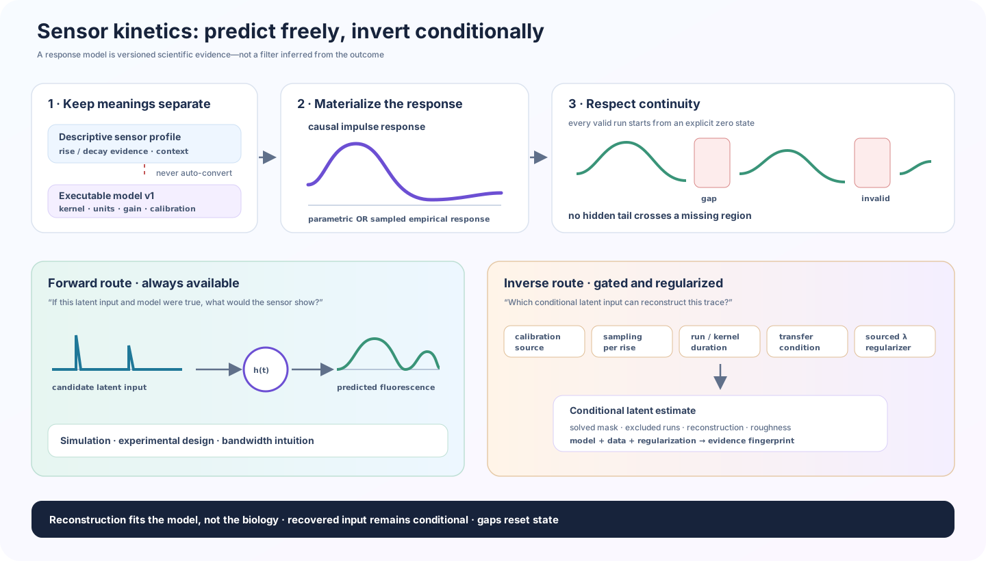
Keep descriptive kinetics separate from an executable model
SensorKinetics in a
versioned sensor profile
records context-specific rise and decay evidence. It deliberately does not say
whether reported values are time constants, 10–90% times, pulse durations,
single-exponential fits or in-vivo impulse responses.
Executable models therefore require a separate identity:
from fiberphotometry import KineticModelIdentity

identity = KineticModelIdentity(
    model_id="lab-dlight13b-pulse-response",
    model_version="1",
    sensor_profile_id="my-lab-dlight13b",
    sensor_profile_version="2026-07-27",
    input_quantity="latent dopamine drive",
    input_unit="calibration a.u.",
    output_unit="dF/F",
    measurement_context="bench pulse calibration",
    evidence_source="calibration protocol and frozen result checksum",
    coefficient_source="independently_calibrated",
    calibration_id="dlight13b-batch-2026-07",
)
An independently calibrated identity requires a calibration ID. Set
coefficient_source="user_declared" for a sensitivity model; it is retained as a
warning and can be made a hard refusal at the deconvolution gate.
The input name and unit describe the calibration model's latent variable. They do not acquire stronger biological meaning when the model is inverted. Use an arbitrary or calibration unit unless an independent concentration calibration actually identifies the gain and response in the relevant preparation.
Choose a causal response family
Difference of exponentials
from fiberphotometry import DifferenceOfExponentialsModel

model = DifferenceOfExponentialsModel(
    identity=identity,
    rise_time_constant_s=0.10,
    decay_time_constant_s=0.50,
    gain=1.0,
    latency_s=0.0,
    tail_fraction=1e-4,
)
This is a causal linear time-invariant sensitivity model. The rise constant must be shorter than the decay constant. Its kernel is normalized to unit area before the declared gain is applied, so a sustained unit input approaches the declared steady-state gain after boundary effects have passed.
Do not copy a profile's descriptive rise and decay numbers into these fields unless the evidence defines them as the corresponding model time constants.
Sampled empirical response
from fiberphotometry import SampledImpulseResponseModel

model = SampledImpulseResponseModel(
    identity=identity,
    sample_interval_s=0.01,
    response_density=tuple(calibrated_impulse_response),
    normalization="unit_area",
    gain=calibrated_gain,
)
This boundary supports an empirical response, an external simulator, or a future
model family without forcing it into the two-exponential shape. The supplied
values are a causal response density beginning at time zero. They are linearly
interpolated onto the recording interval. unit_area separates shape from gain;
as_supplied preserves the response integral exactly.
kinetic_kernel(model, sampling_interval_s) materializes the exact density and
discrete convolution weights used by either route, including integral, peak time
and finite support.
Run the forward model first
from fiberphotometry import KineticForwardSpec, predict_sensor_response

prediction = predict_sensor_response(
    time_s,
    candidate_latent_input,
    model,
    KineticForwardSpec(),
    valid=latent_valid,
)
Forward prediction is the easier and usually more defensible question: “If this latent input and model were true, what output would be observed?” It is useful for simulation, experimental-design checks and testing whether proposed biological dynamics survive the sensor's bandwidth.
Timestamp gaps, invalid input and non-finite samples split continuity runs. Each
run begins with a declared zero model state. No tail is carried across a gap.
boundary_affected_sample_count makes the samples whose prediction depends on
that zero-state assumption visible; they are not silently presented as steady
state.
Assess identifiability before looking at the inverse
from fiberphotometry import (
    KineticDeconvolutionSpec,
    assess_kinetic_identifiability,
)

inverse_spec = KineticDeconvolutionSpec(
    regularization_strength=1e-4,
    regularization_source="held-out calibration reconstruction",
    smoothness_order=1,
    nonnegative=True,
    fit_run_baseline=True,
    minimum_samples_per_rise=3,
    minimum_run_to_kernel_ratio=2,
    require_independent_calibration=True,
)

assessment = assess_kinetic_identifiability(
    time_s,
    model,
    inverse_spec,
    valid=signal_valid,
)
assessment.require_ready()
This assessment is outcome-blind. It checks:
- whether coefficients are independently calibrated or user-declared;
- samples per rise time constant for the parametric model;
- each uninterrupted run's duration relative to kernel support;
- the unregularized and regularized transfer condition numbers;
- the frequency range retaining the declared fraction of maximum transfer; and
- the maximum gain of the selected regularized inverse filter.
Under-sampled rise dynamics, an unresolved transfer nullspace, an excessive
regularized condition number, or no eligible run produces status="fail".
Short individual runs and an assumed model remain explicit warnings. Supplying a
positive regularization value is mandatory: an unregularized inverse is not an
available accidental default.
Transfer diagnostics describe numerical recoverability under the model. They do not measure in-vivo noise, model mismatch, motion, hemodynamics or saturation. Run sensor and reference validity and any relevant optical unmixing before this stage.
Estimate a conditional latent input
from fiberphotometry import deconvolve_sensor_response

result = deconvolve_sensor_response(
    time_s,
    observed_dff,
    model,
    inverse_spec,
    valid=signal_valid,
)
The solver minimizes reconstruction error plus the declared zeroth-, first- or
second-order penalty. nonnegative=True applies a nonnegative bound to the latent
input while leaving each run's optional baseline unconstrained.
Each eligible continuity run is solved independently. The result retains:
- the latent estimate and reconstructed output on the original timestamp grid;
- a
solvedmask, with excluded runs leftNaNrather than interpolated; - fitted run baseline, RMSE, R² and reconstruction correlation;
- latent roughness, lower-bound activity and solver iterations;
- kernel-boundary exposure for every solved run;
- the complete identifiability assessment; and
- an evidence fingerprint binding data, masks, model and inverse specification.
High reconstruction R² is necessary but weak evidence: a flexible regularized inverse can reconstruct data under a misspecified kernel. It is not a model validation statistic and is not an uncertainty interval.
Treat regularization as a robustness choice
Regularization controls the scientific answer. A small value may amplify noise
and create narrow events; a large value may merge events and attenuate amplitude.
The package therefore requires a named regularization_source and binds the value
into the evidence fingerprint.
Prefer a value frozen from independent calibration or simulation. When several values remain defensible, run named specifications and report whether timing, integrated input and condition contrasts survive the set. Do not choose the value that makes the biological result most attractive. A typed cross-regularization summary and calibrated latent uncertainty remain roadmap work.
Current claim boundary
Available now:
- versioned calibrated or user-declared model identity;
- parametric and sampled causal linear response families;
- gap-bounded forward prediction with boundary evidence;
- outcome-blind sampling, duration and transfer diagnostics; and
- regularized unconstrained or nonnegative inversion with full reconstruction evidence.
Still deliberately unresolved:
- nonlinear binding, saturation, bleaching or time-varying kinetics;
- automatic conversion from descriptive sensor-profile kinetics;
- automatic regularization selection from the biological outcome;
- calibrated latent-input uncertainty;
- universal sensor coefficients supplied by the package; and
- concentration claims without an independent preparation-relevant calibration.
The decision is recorded in SDR-0054.