Multiscale summaries for long recordings

Use this workflow when the question is how a processed photometry signal changes over seconds, minutes, or longer periods, and no single event defines the analysis. It emits observable window summaries; it does not infer a biological “tonic” or “phasic” component from window length.

This is an experimental product API. It accepts irregular timestamps in physical time, keeps gaps and supplied state epochs as hard boundaries, exposes every window denominator, and carries one chosen summary through session-to-animal inference.

Scales describe observation windows, not biology. Every candidate window retains coverage and acceptance evidence. Inferential comparisons aggregate windows within sessions and sessions within animals before resampling animals.

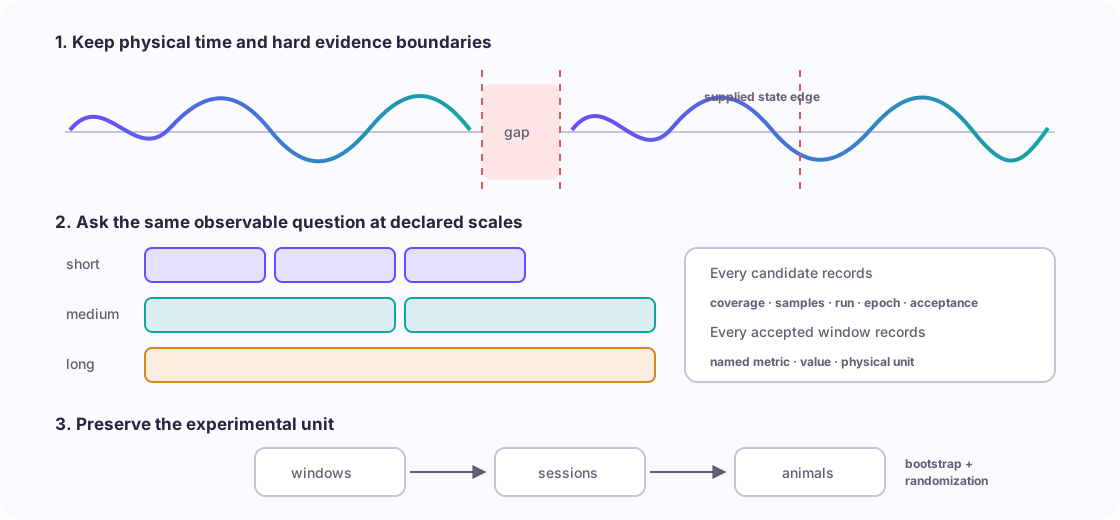
What is available

Need	Public contract	Evidence retained
Several physical-time scales	MultiscaleWindowSpec	name, duration, step, minimum coverage and samples
Gap-aware, optionally state-conditioned summaries	summarize_multiscale	continuity runs, epoch identity, accepted and rejected windows
Irregular-sampling-aware location and spread	time_weighted_* metrics	trapezoidal physical-time integration and observed duration
Familiar sample descriptions	sample_* metrics	explicit sample weighting and sample count
Animal-level condition contrasts	infer_multiscale_animals	window→session→animal ledger, interval and randomization test

Declare scales and observables

from fiberphotometry import (
    MultiscaleContinuitySpec,
    MultiscaleSummarySpec,
    MultiscaleWindowSpec,
    summarize_multiscale,
)

summary_spec = MultiscaleSummarySpec(
    windows=(
        MultiscaleWindowSpec(
            "ten_seconds",
            duration_s=10,
            step_s=5,  # 50% overlap is explicit
            minimum_coverage=0.95,
            minimum_samples=20,
        ),
        MultiscaleWindowSpec(
            "five_minutes",
            duration_s=300,
            step_s=300,  # non-overlapping
            minimum_coverage=0.98,
            minimum_samples=300,
        ),
    ),
    metrics=(
        "time_weighted_mean",
        "time_weighted_standard_deviation",
        "sample_median",
        "sample_iqr",
        "sample_linear_slope",
    ),
    continuity=MultiscaleContinuitySpec(
        gap_factor=3,
        maximum_gap_s=None,
    ),
)

result = summarize_multiscale(
    time_s,
    processed_signal,
    summary_spec,
    valid=valid_samples,
    value_unit="dF/F",
)

When step_s is omitted, it equals duration_s. A smaller step creates overlapping estimates; a larger step intentionally leaves unsummarized time. The window duration remains the coverage denominator even at a recording edge, so an incomplete final window is not made to look complete by shortening its target.

Choose weighting deliberately

The metric name says what receives equal weight:

Metric	Calculation	Unit
time_weighted_mean	trapezoidal integral divided by observed seconds	signal unit
time_weighted_standard_deviation	physical-time weighted variation around the time-weighted mean	signal unit
time_weighted_rms	physical-time weighted root mean square	signal unit
sample_mean, sample_median	each acquired sample has equal weight	signal unit
sample_standard_deviation, sample_iqr, sample_rms	sample-weighted spread or magnitude	signal unit
sample_linear_slope	least-squares signal change per clock second	signal unit/s

Time-weighted metrics linearly interpolate only between adjacent observations inside one continuity run. They do not interpolate across a missing sample, acquisition gap, or state boundary. Sample metrics remain useful after prospective regularization or when matching a published sample-based estimand, but their names prevent an irregular clock from silently changing temporal weighting.

Inspect acceptance before values

accepted = [window for window in result.windows if window.accepted]
rejected = [window for window in result.windows if not window.accepted]

for window in rejected[:5]:
    print(
        window.scale,
        window.coverage_fraction,
        window.sample_count,
        window.exclusion_reason,
    )

for run in result.runs:
    print(run.run_id, run.state, run.epoch_id, run.interval_cv)

Each MultiscaleEstimate points back to one window_id. The corresponding MultiscaleWindowRecord supplies the run, physical bounds, sample count, observed duration, coverage, and acceptance decision. Rejected candidates remain in the ledger but produce no estimate. Isolated valid segments with fewer than two samples remain in run_exclusions, because they cannot support physical-time integration. evidence_fingerprint binds the signal, validity, epochs, units, scales, metrics, and continuity policy.

Condition on externally supplied states

from fiberphotometry import StateEpoch

epochs = (
    StateEpoch("exploration", 12.0, 48.5, epoch_id="bout-001"),
    StateEpoch("rest", 55.0, 91.0, epoch_id="bout-002"),
)

by_state = summarize_multiscale(
    time_s,
    processed_signal,
    summary_spec,
    valid=valid_samples,
    epochs=epochs,
    value_unit="dF/F",
)

Epochs are half-open and may not overlap. Equal state labels in separate epochs remain separate continuity runs. Samples outside supplied epochs are counted in unassigned_valid_sample_count; the package does not discover or fill state.

Compare conditions across animals

Attach identity only after each session has been summarized:

from fiberphotometry import (
    MultiscaleAnimalInferenceSpec,
    MultiscaleStudySession,
    infer_multiscale_animals,
)

sessions = [
    MultiscaleStudySession(
        subject="mouse-01",
        session="day-01",
        condition="vehicle",
        result=mouse_01_day_01,
    ),
    # More independently acquired sessions and animals...
]

contrast = infer_multiscale_animals(
    sessions,
    MultiscaleAnimalInferenceSpec(
        scale="five_minutes",
        metric="time_weighted_mean",
        condition_a="vehicle",
        condition_b="drug",
        state="rest",  # use None for an unconditioned result
        design="paired",
        effect_scale="difference",
        window_aggregation="median",
        session_aggregation="median",
        seed=2026,
    ),
)

The reported difference is condition B minus condition A; a ratio is B/A. Windows are aggregated within each session, then sessions receive equal weight within each animal. Bootstrap samples and paired swaps or independent-label permutations act on animals. summed_window_observed_duration_s is an evidence total and can exceed recording duration when windows overlap; it is never treated as the number of independent replicates.

Relationship to the rest of the toolkit

• Use spontaneous-transient analysis when the estimand is event rate, amplitude, width, or area.
• Use time, frequency, and state analysis for autocorrelation, PSD, spectrograms, coherence, or band power. Fourier methods require a regular clock; physical-time multiscale integration does not.
• Run across-session comparability before treating a change in scale summaries as longitudinal biology.
• Pass declared, comparable session summaries to Unspool for learning trajectories rather than rebuilding behavioral longitudinal models here.

Boundaries and open validation

This workflow does not estimate a latent baseline, deconvolve sensor kinetics, identify sustained neurotransmitter release, discover states, or choose a biologically privileged scale. Absolute mean and slope can remain sensitive to bleaching, motion, hemodynamics, reference correction, and session-to-session scale changes. Reasonable scales and weighting choices therefore belong in a named multiverse when the conclusion depends on them.

The API is experimental until it has raw-signal and annotation validation across multiple sensors and acquisition systems. See SDR-0051 for the decision and alternatives.