Population inference for frequency and lag curves v0.1
Use this experimental workflow when the outcome is a complete one-dimensional curve—rather than a prespecified scalar band or lag—and the population question is defined across animals.
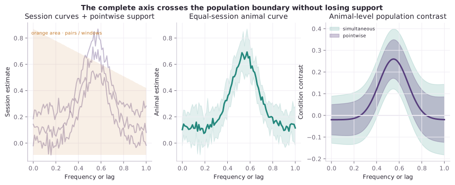
Supported curves
| Session result | Adapter | Axis | Pointwise lower-level support |
|---|---|---|---|
WelchPSDResult |
curve_session_from_psd() |
frequency in Hz | complete Welch windows at every frequency |
AutocorrelationResult |
curve_session_from_autocorrelation() |
lag in seconds | valid within-run pairs at each lag |
LaggedAssociationResult |
curve_session_from_lagged() |
lag in seconds | jointly valid within-run pairs at each lag |
CoherencePhaseResult |
curve_session_from_coherence() |
frequency in Hz | complete joint Welch windows at every frequency |
The coherence adapter materializes magnitude-squared coherence. It does not average phase angles; population phase requires a separately validated circular estimand.
Adapt sessions
Single-signal PSD results do not contain experimental identities, so attach them explicitly:
from fiberphotometry import curve_session_from_psd

session_curve = curve_session_from_psd(
    psd_result,
    subject="mouse-01",
    session="day-01",
    level="post",
)
Lagged association and coherence results already contain subject, session, and pair identity. Only the experimental level is added:
from fiberphotometry import (
    curve_session_from_coherence,
    curve_session_from_lagged,
)

lag_curve = curve_session_from_lagged(lagged_result, "post")
coherence_curve = curve_session_from_coherence(coherence_result, "post")
The metric identifier includes the declared signal-pair ID, preventing curves from different channel/site pairs from being pooled accidentally.
State-conditioned helpers
Externally supplied state outputs can be expanded without relabeling them:
from fiberphotometry import (
    curve_sessions_from_state_autocorrelation,
    curve_sessions_from_state_coherence,
    curve_sessions_from_state_psd,
)

psd_curves = curve_sessions_from_state_psd(state_psd_session)
acf_curves = curve_sessions_from_state_autocorrelation(
    state_autocorrelation,
    subject="mouse-01",
    session="day-01",
)
coherence_curves = curve_sessions_from_state_coherence(state_coherence)
Each supplied state label becomes a population level. The helper does not discover, merge, or reinterpret states.
Materialize animal curves
from fiberphotometry import (
    PopulationContrastSpec,
    materialize_curve_population,
)

materialized = materialize_curve_population(
    session_curves,
    levels=("pre", "post"),
    session_aggregation="mean",
)

population = materialized.contrast(
    PopulationContrastSpec(
        numerator="post",
        denominator="pre",
        design="paired",
        draws=2_000,
        seed=2026,
    )
)
Sessions are aggregated pointwise within each animal-level cell. At every axis point, the result retains:
- the number of finite contributing sessions in
support; - the summed valid pairs or complete windows in
observation_support; - pointwise animal counts in the population result; and
- the contributing session IDs.
Pairs and windows never determine population weight. Two animals remain two population units even if one has far more valid samples.
The materializer averages already-computed session curves equally; it does not re-pool raw auto-spectra or cross-spectra across sessions. For coherence, the estimand is therefore the animal's equal-session mean magnitude-squared coherence on its native bounded scale. Exposure-weighted pooling, variance-stabilizing transforms, and cross-spectrum-first animal estimands remain explicit alternatives rather than hidden defaults.
Exact-axis policy
Every selected session must have the identical ordered axis, metric, axis unit, and
value unit. A changed sampling rate, maximum lag, Welch window, or frequency limit
usually changes that grid. materialize_curve_population() refuses the mixture
with an instruction to harmonize prospectively.
There is no implicit interpolation, truncation to overlap, or nearest-bin matching. If a common grid is scientifically justified, construct it as an explicit upstream operation and retain that operation in provenance before adapting the curves.
Whole-axis uncertainty
The common population result contains both pointwise intervals and a simultaneous max-t band over the declared complete axis. The simultaneous band is the relevant default when inspecting the curve to find where an effect appears largest. It does not identify a frequency band, lag interval, onset, or peak without a separate selection rule.
The same materialization supports the two-group × two-condition interaction:
This forms a complete within-animal condition-difference curve before comparing those curves between disjoint groups.
Current boundary
- The common estimand is additive: numerator minus denominator.
- Axes are one-dimensional. Spectrogram matrices require a separate two-dimensional support and multiplicity contract.
- Coherence is supported; phase, cross-power components, and directed connectivity are not population-averaged here.
- PSD magnitude is comparable only when signal units, preprocessing, sampling, and spectral specifications are comparable upstream.
- The bootstrap calibration assumptions and small-sample limitations of the common population layer still apply.
- Choosing a frequency range, lag range, state definition, smoothing rule, or preprocessing family remains a prospective scientific decision.
The governing rationale is recorded in SDR-0058.